Biped Robot – Dynamic Model

I wanted to develop a mathematical model of the biped’s leg to allow me to:

Help spec the motors needed for each joint
Refresh and relearn solid kinematics and dynamics
Refresh and relearn Matlab (hadn’t properly used it in 12 years)

Rough proportions were based off the Star Wars Galaxy BD-X robot.
I set a height of 400mm (to limit how large it gets) and adjusted geometry of the different until it either looked close for me to start with.

The Leg

The leg consisted of 6 main sub-assemblies:

A femur (upper leg)
A tibia (lower leg)
A foot
Drive methods for each (3 in total)

Based off of some readings on Josh Pieper’s Quadruped, and Ben Katz’s Mini Cheetah, I wanted to put motors for knee and hip coaxially at the hip.
This helps minimise the rotational inertia around the hip. The joints won’t be moving fast but seems good practice.
The foot added complexity, needing another drive method (active or passive) to manipulate it.
To simplify initial designs I decided to remove the articulating foot and will rely on the end of the tibia as an acting foot.
As the design progresses I hope to bring an articulating foot back into the design. It makes it look a bit more complete, and may help with stability when standing in a spot.
I’ll cover more details in a separate post on the leg design.

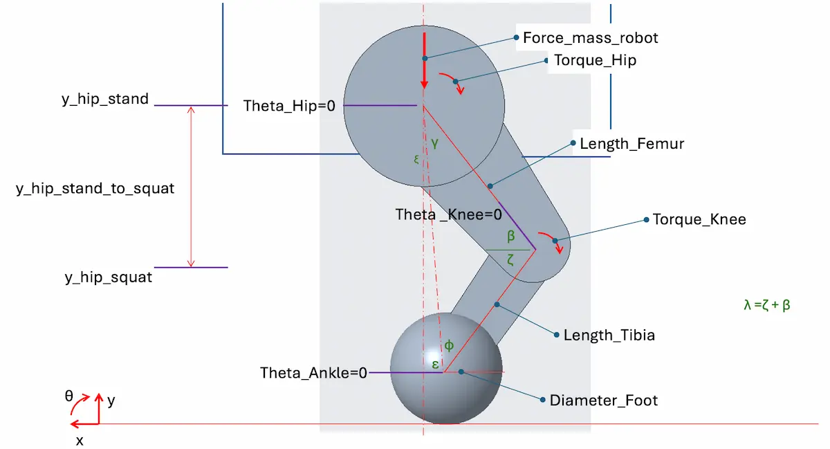
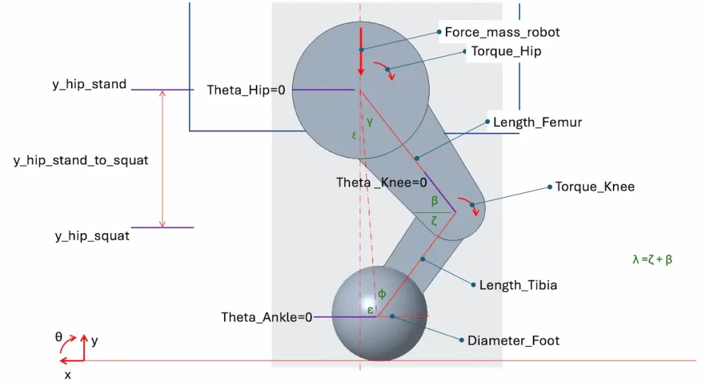
To transform this into a dynamic model, I defined coordinate systems and variables per below.
Each limb, could be separated for defining free body and kinetic diagrams.

Definition of leg coordinates, and symbols

Program Overview

The sequence of the dynamic model is below.
I would like to have it able to sweep through a range of variables that are currently constant to get a clearer understanding of the impact of each (for example, mass). Alternatively, I could also narrow the computation scope and run it in a Design of Experiment (DoE) format.

Load all constants
Calculate hip acceleration, velocity, and position profiles and values
Calculate joint angles
Calculate knee positions
Calculate joint angular velocities and angular accelerations
Calculate tibia CoG and knee linear accelerations
Calculate femur angular velocity and accelerations
Calculate femur CoG accelerations
Define the kinetic array, K (dynamic or static)
Define the force matrix, H
Define the constant force array, f
Solve for the forces and torques
Calculate instantaneous powers
Generate plots and tables

Constants

With the basic geometry and leg architecture “set” the remaining parameters for the model were defined and set. These could all be adjusted and the simulation re-run.

A time step: 0.001s
Total robot mass: 4kg (an initial rough estimate)
Leg limb masses, rotational inertias, and COGs: Values calculated off of rough CAD with PLA properties
Motor masses and rotational inertias: Initial values based on Mini Cheetah, later updated to the chosen motor’s.
Movement profile: This was a rough squat to stand movement
- Squat hip position: 70mm above a reference plane through the ankle axis
- Standing hip position: 155mm above a reference plane through the ankle axis
- Time from squat to stand: 2s – initial value which I could easily change based on results
- Velocities and accelerations at start and point both zero.
- Motion was vertical only

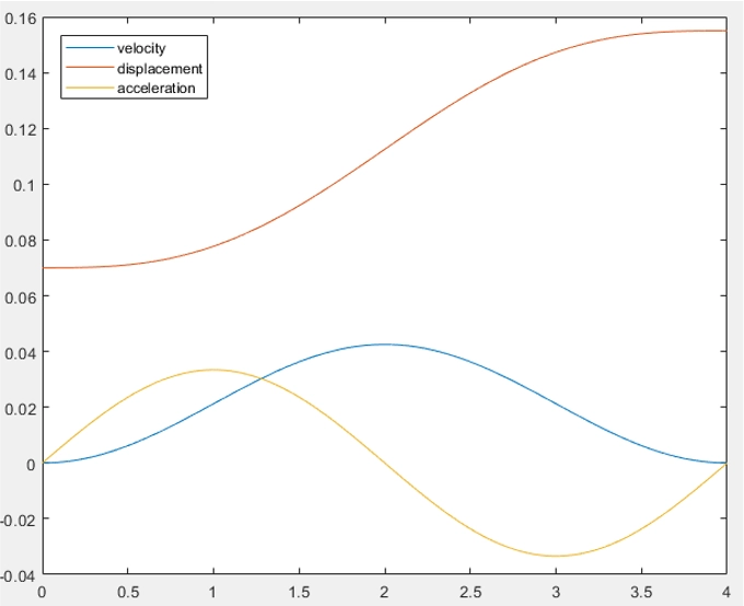
Hip linear accelerations, velocities, and displacements

Having a smooth transition from acceleration to deceleration was achieved by relying on a sinusoidal motion equation.
Initial profiles had a triangle form for velocity which lead to discontinuities, and impacted the subsequent calculations.
The profile calculation would update profile equation coefficients based on travel time, and start and end position variables.

Motion profiles for 4s; displacement(orange), velocity (blue), and acceleration (yellow)

Knee and Hip Calculations

Constraining the ankle in place at (0, 0), and treating it as a pin joint, the knee positions and joint angles can be determined as a triangle through ankle-knee-hip.

From knowing the hip and knee angles for each time step we can calculate angular velocities and accelerations from the differences across each time step.

Tibia CoG and Knee linear accelerations

With the tibia motion being fixed at (0, 0) and now having tibia angular acceleration (about the ankle) we can easily determine tibia CoG and Knee accelerations.
By their distance from the ankle axis, it’s a transform from rotational coordinates to Cartesian.

Femur angular velocity and accelerations

The femur motion is a combination of rectilinear translation and rotation.
We know the translation from the hip motion, the rotation we can determine from the knees motion that we’ve already calculated.

$\begin{bmatrix} a_{Hx} \\ a_{Hy} \\ \end{bmatrix} = \begin{bmatrix} -L_T\sin(\theta_A) & -L_T\cos(\theta_A) & L_H\sin(\theta_H) & L_H\cos(\theta_H) \\ L_T\cos(\theta_A) & -L_T\sin(\theta_A) & -L_H\cos(\theta_H) & L_H\sin(\theta_H) \\ \end{bmatrix} \begin{bmatrix} \alpha_{AK} \\ \omega^2_{AK} \\ \alpha_{KH} \\ \omega^2_{KH} \\ \end{bmatrix}$

All are known except for femur angular velocity and angular acceleration.

Femur CoG Accelerations

Knowing the femur angular motions we can calculate for any point on its body. The equation is used but with scaling for the femur length. q is the ratio for where the femur’s centre of gravity along its length.

$\begin{bmatrix} a_{FGx} \\ a_{FGy} \\ \end{bmatrix} = \begin{bmatrix} -L_T\sin(\theta_A) & -L_T\cos(\theta_A) & (q-1)L_H\sin(\theta_H) & (q-1)L_H\cos(\theta_H) \\ L_T\cos(\theta_A) & -L_T\sin(\theta_A) & (1-q)L_H\cos(\theta_H) & (q-1)L_H\sin(\theta_H) \\ \end{bmatrix} \begin{bmatrix} \alpha_{AK} \\ \omega^2_{AK} \\ \alpha_{KH} \\ \omega^2_{KH} \\ \end{bmatrix}$

Equations of Motion

We now have all the information to calculate the unknown forces. Equations of motion are needed to define how the forces are related and dependent with respect to the system.
The equations were first created individually per body then transformed into the appropriate sections of the Kinetic array (K), Force matrix (H), and Constant force array (f) for solving.
Each of these were unique per time step as they are dependent on joint angles.

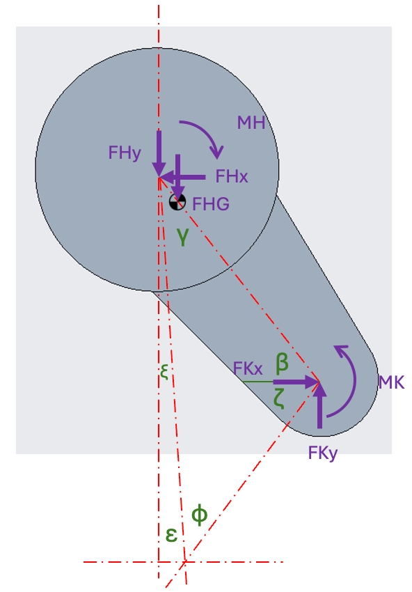
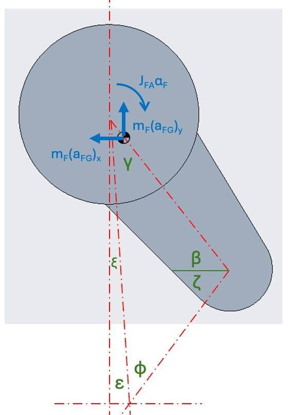
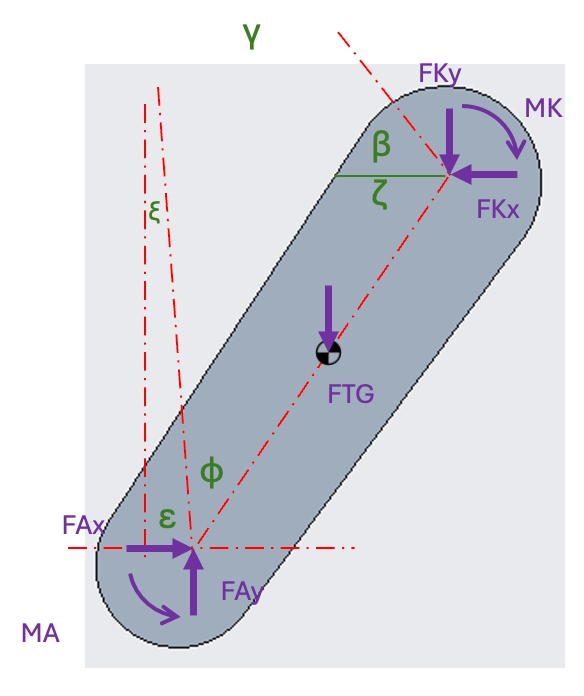
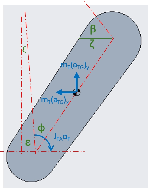
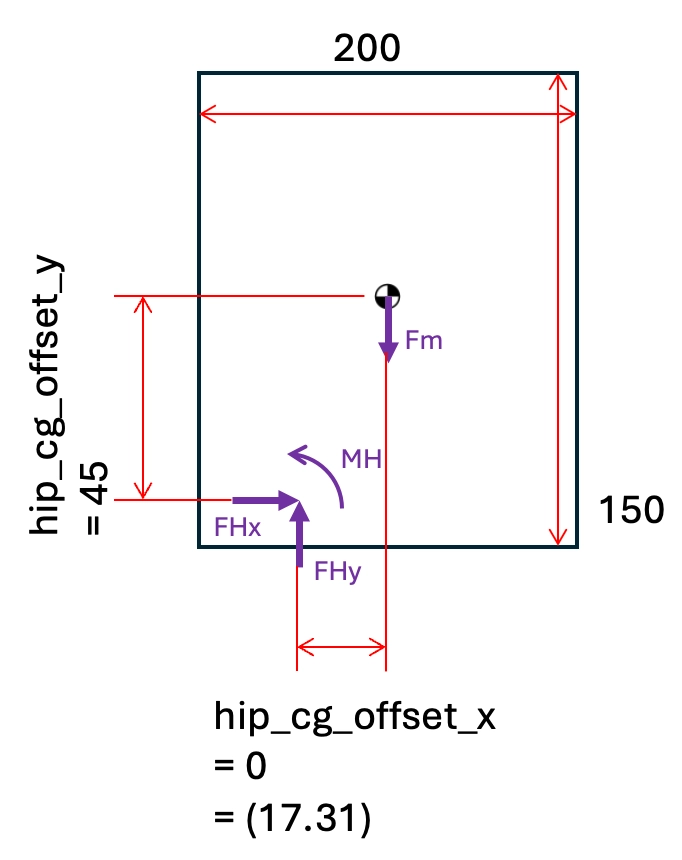
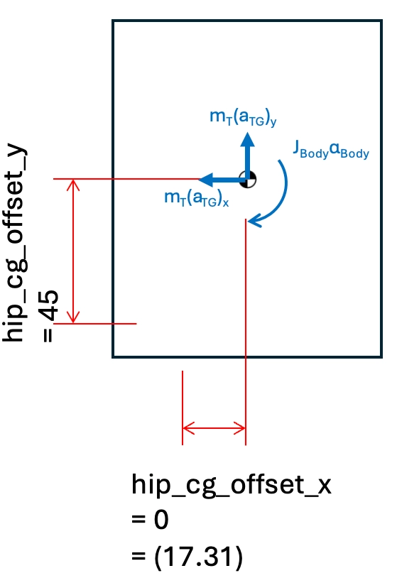
These are ordered in the arrays and matrix as the following:

$\begin{bmatrix} Femur Forces in x // Femur Forces in y // Tibia Forces in x // Tibia Forces in y // Body Forces in x // Body Forces in y // Body Moments about COG // Tibia Moments about Knee // Femur Moments about CoG // \end{bmatrix}$

Kinetic Array

I created two kinetic arrays, one including dynamics from the limb’s masses and rotational inertias, the other with static only (i.e. accelerations are zero).
The dynamic kinetic array is:

${\begin{bmatrix} a_{femur_g,x} m_{femur} \\ a_{femur_g,y} m_{femur} \\ a_{tibia_g,x} m_{tibia} \\ a_{tibia_g,y} m_{tibia} \\ 0 \\ a_{hip,y} (m_{total}-m_{leg}) \\ 0 \\ J_{tibia\_g}\alpha_{ankle}+nL_{tibia}m_{tibia}(\sin(\zeta)a_{tibia\_g,x}+\cos(\zeta)a_{tibia\_g,y})) \\ J_{femur_g}\alpha_{femur} \\ \end{bmatrix}}$

Force Matrix

The 9×8 force matrix consists of the coefficients for the various unknown forces in the equations of motions.

Constant Force Array

The constant force arrays consists of all the forces and moments that independent of the unknowns that we’re solving for.

${\begin{bmatrix} 0 \\ -FHG \\ 0 \\ -FTG \\ 0 \\ -(mass_{total}-mass_{leg}) \\ 0 \\ -FTG.n.L_{Tibia}*\cos\left(\zeta\left(i\right)\right) \\ 0 \\ \end{bmatrix}}$

Solving

The equations of motion in the form ΣF=ma or its rotational equivalent is:

${HF + f= K}$

and in the form we need Matlab to solve is

$F=H^{-1}\left(K-f\right)\equiv H\space\backslash\left(K-f\right)$

This gives us arrays (one per time step) for:

Hip forces in x and y
Knee forces in x and y
Ankle forces in x and y
Moments on the Hip
Moments on the Knee

Power

Instantaneous power is simply the moment multiplied by the relevant angular velocity for each time step.
This is helpful for sizing the motors and any power transmissions.

Plots and Tables

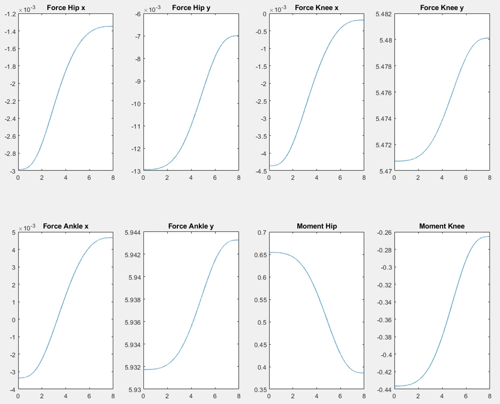
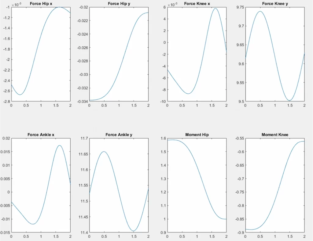
Plots were generated for the different forces and moments solved to help visualise how these changed, where peak values were (an in what context), and which forces or moments were significant.
Tables were also made to clearly quantify what max, min, and mean values were for each.
See some plots here.

Forces and Moments for 4kg robot mass and 2s movement time

Learnings along the way

Initial rotational inertias for the limbs were entered with the wrong units which lead to results a magnitude out.
This lead to thinking higher power, current, and torques were present.
Thankfully, this lead to designing for values larger than the corrected results show so can continue knowing I should have a larger factor of safety than initially intended.
If it was the other way round then I would have probably needed new motors.

As the design changes, for example adjusting tibia structure, then masses and inertias can get updated and the analysis re-run to confirm any impact.

Source

I plan to make the source available. Once I have added it to github with appropriate licenses, I’ll add a link to this post.

Matter Evolved